Principles of singular value decomposition
Linear algebra background
In vector algebra, linear transformations are defined as the transformation of a vector with stretching, squishing, shearing, or rotating by tracking basis vector movements.
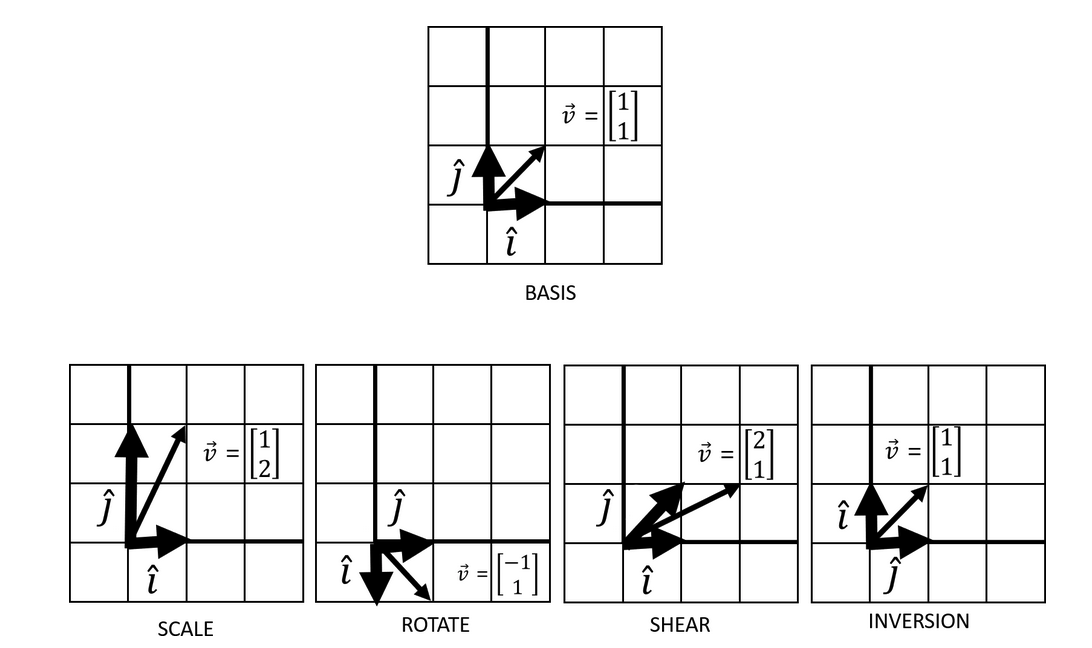
This transformation of a given vector by the application of basis vectors is the concept of vector matrix multiplication. This is easily seen when we think of the basis vectors as packaged into a matrix. Think of this simple example where we transform a given vector \(v_{i}\) by the transformation of basis vector \(\hat{i}\) by a factor of 2 and \(\hat{j}\) by a factor of 4:
\[ \left(\begin{array}{cc} 2 & 0\\ 0 & 4 \end{array}\right) \left(\begin{array}{cc} x_{i}\\ y_{i} \end{array}\right) \]
This is the most simplest case where the vector \(v_{i}\) is elongated by the scaled basis vectors \(\hat{i}\) and \(\hat{j}\). That is, this constitutes a single linear transformation. But what if we were to chain multiple linear combinations together? The consolidation of multiple linear transformations constitute a matrix multiplication task.
\[ AB = \left(\begin{array}{cc} a & b\\ c & d \end{array}\right) \left(\begin{array}{cc} e & f\\ g & h \end{array}\right) = \left(\begin{array}{cc} ae + bg & af + bh\\ ce + dy & cf + dh \end{array}\right) \]
Above, two matrices \(A\) and \(B\), each representing a linear transformation (whether that's elongation, inversion, rotation...) were consolidated by a matrix dot product. Multiplying this 2x2 matrix \(AB\) to a given vector \(v_{i}\) via vector-matrix multiplication would result a new transformed vector. An important note here is that matrix dot product is not commutative - that is, the order of the linear transformations matters. Regardless, it is clear that matrices represent some combinations of linear transformations.
Principles of SVD
Given an \(m\) by \(n\) matrix \(A\), let's say there exists a pair of orthogonal vectors that remain orthogonal after transformation by \(A\). In two dimensions, this is saying:
\(Av_{1} = y_{1}\) and \(Av_{2} = y_{2}\)
Of course, a vector constitutes a magnitude and a direction. This is analogous to the concept of stretching a basis vector of unit 1 (direction) by a scalar factor (magnitude). This means that the above expressions can be written as:
\(Av_{1} = \sigma u_{1}\) and \(Av_{2} = \sigma u_{2}\)
In matrix form:
\(A[v_{1}, v_{2}] = [\sigma u_{1}, \sigma u_{2}]\)
\(A[v_{1}, v_{2}] = [u_{1}, u_{2}] \left(\begin{array}{cc}\sigma_{1} & 0\\0& \sigma_{2}\end{array}\right)\)
Which, using matrix notation equals to:
\(AV = U\Sigma\)
The fact that for every \(m\) by \(n\) matrix \(A\) the above equation is satisfied is the core basis of singular value decomposition (SVD). In context of SVD, it's helpful to rearrange the equation in context of deconstructing \(A\) into three parts:
\(A = U\Sigma V^{T}\)
Since we've made it clear that a matrix can be thought of a composition of linear transformations, the above expression dictates that the linear transformations can be decomposed into its constituent parts. The three parts are:
- \(V\) = a \(n\) by \(n\) matrix describing a rotation in the input space.
- \(\Sigma\) = a \(m\) by \(n\) diagonal matrix describing a scaling factor that takes the vector into output space.
- \(U\) = a \(m\) by \(m\) matrix describing a rotation in the output space.
The following are then true:
- Both \(V\) and \(U\) are orthogonal, as stated before.
- \(V^{T}V = I\) and \(U^{T}U = I\) must be true since they are orthogonal and this indicates these are rotation matrices.
- \(\Sigma = diag(\sigma)\).
- The trace of the diagonal matrix \(\Sigma\) is the sum of the values in the diagonal \(\sigma\).
- \(\sigma_{1} \ge \sigma_{2} \ge ... \ge \sigma_{r} \ge 0\) where \(r\) is the rank of \(A\).
The diagram below visually shows the decomposition of the transformation given by A on a vector into its constituent parts:
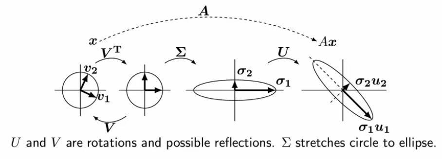
The diagonal values \(\sigma\), which describe the extent of stretching of the transformation, are called the singular values of A. Largest values of \(\sigma_{i}\) indicate the largest scaling factor in the dimension \(i\). The vectors \(V\) and \(U\) are called left and right singular vectors, respectively.
Why is this important? The decomposition of matrices can be used in principal component analysis (PCA), which I will cover shortly. However, SVD can also be used for low-rank approximation. This means that we can use SVD to use a truncated version of the original data matrix \(A\) by some matrix \(B\).
Remember that according to SVD, \(A = U\Sigma V^{T}\) and \(\Sigma\) contains singular values \([\sigma_{1}, ..., \sigma_{r}]\) where \(r\) is the rank of A. However, since \(\sigma_{1} \ge \sigma_{2} \ge ... \ge \sigma_{r} \ge 0\) is true (that is, the magnitude of the singular values decay), there exists a set of singular values \([\sigma_{1}, ..., \sigma_{k}]\) where \(k < r\) that provides a good approximation of the original matrix.
This means that we can set the smallest \(\sigma\) values to zero in \(\Sigma\) to obtain the truncated version \(\tilde{\Sigma}\). This means:
\(\tilde{\Sigma} = diag(\sigma_{i})\) where \(i = 1, ..., k\)
And:
\(B = U\tilde{\Sigma} V^{T}\).
The truncated matrix \(B\) that best approximates \(A\) is said to be the best rank \(k\) approximation of \(A\) given that the Frobenius norm of the difference between \(A\) and \(B\) is minimized. That is:
\(min_{B} ||A-B||_{F}\) where \(rank(B) = k\)
SVD and eigendecomposition
The eigendecomposition of a square matrix \(A\) is defined as:
\(Av_{i} = \lambda_{i}v_{i}\), where:
- \(\lambda_{i}\) are real numbers and are called the eigenvalues and
- \(v_{i}\) are orthogonal vectors and are called the eigenvectors.
Remember that in context of SVD, we were considering non-square matrices of shape \(m\) by \(n\) and thus the eigendecomposition does not satisfy. However, it turns out that the matrix multiplication between an \(m\) by \(n\) matrix and its transpose yields a square matrix. What is the importance of this?
Let's go back to the SVD expression:
\(A = U\Sigma V^{T}\)
Let's multiply each side by the transpose of \(A\) from the left side to get:
\(A^{T}A = (V \Sigma^{T} U^{T} ) (U \Sigma V^{T})\)
We know that \(U\) is an orthogonal matrix and thus \(U^{T}U = I\). This means:
\(A^{T}A = V \Sigma^{T} \Sigma V^{T}\)
Remember that \(\Sigma\) is a square diagonal matrix. This means that \(\Sigma \Sigma^{T}\) contains simply the square of the individual diagonal values, that is, \(diag(\sigma^{2})\).
The above equation may look familiar because it's just the eigendecomposition of \(A^{T}A\); the eigenvalues are the squared singular values \(\sigma\) of \(A\) and the eigenvectors are vectors in \(V\).
Since we know matrix multiplication is not commutative, we also need to check out what happens when we multiply by the transpose of A from the right side:
\(AA^{T} = (U \Sigma V^{T}) ( V \Sigma^{T} U^{T})\)
Similarly, since \(V\) is an orthogonal matrix:
\(AA^{T} = U \Sigma \Sigma^{T} U^{T}\)
Therefore, the eigenvalues of \(AA^{T}\) are once again the squared singular values \(\sigma\) of \(A\) but this time the eigenvectors are vectors in \(U\).
SVD and PCA
So far we've concluded that an \(m\) by \(n\) matrix \(A\) can be decomposed into \(U\Sigma V^{T}\) and that the square matrices \(A^{T}A\) and \(AA^{T}\) have the corresponding eigenvectors \(V\) and \(U\), respectively. We've also seen that the squared diagonal elements \(\sigma\) of \(\Sigma\) are the corresponding eigenvalues.
Interestingly, it turns out that for a matrix \(A\) - if and only if \(A\) is centered - its covariance matrix can be expressed as such:
\(C = \frac{1}{n-1} AA^{T}\)
This means that the covariance matrix \(C\) can be estimated using the matrix \(AA^{T}\). The covariance matrix by definition is symmetric and diagonalizable, such that eigendecomposition can be applied.
We saw above that the eigenvectors of \(AA^{T}\) - that is, the estimation of covariance matrix \(C\) - are contained in \(U\). The eigenvalues are described by the square of \(\sigma_{i}\). Since instead of a data matrix we're working with a covariance matrix, it must be then:
- The eigenvalues \(\sigma_{i}^{2}\) describes the extent of variance in \(i\)
- The eigenvectors \(u_{i}\) in \(U\) describes the dimension in which the variance is projected on
Therefore, if we're interested in selecting the first \(k\) dimensions that describe the most variance in our original data matrix \(A\), we'd select the first \(k\) eigenvectors and the sum of \([\sigma_{1}^{2}, .... \sigma_{k}^{2}]\) describe the total variance explained. This is the core concept of dimensionality reduction by PCA - projecting high-dimensional data into a lower set of dimensions while maximizing variance explained in the data.
Image credits: 1. 'Essential Math for Data Science' by Thomas Nield (published by O'Reilly Media Inc.) 2. 'Singular value decomposiiton (SVD)' by Gilbert Strang (posted by MITOpenCourseWare on their YouTube channel)