L1, L2 norms and regularized linear models

May 30, 2022 · 6 min read

Bias and variance

The bias-variance tradeoff describes the problem in balancing the two types of errors in supervised learning models. This conflict arises from the model's estimated parameters learned from the training data and its ability to generalize beyond this data. In short, bias describes the assumptions made by the model in regards to the target function; a low-bias model makes less assumptions while a high-bias one makes more. High-bias models are generally less flexible for this reason. Examples of such models include linear models and logistic regression.

On the other hand, variance describes the extent of influence the changes in training dataset has on the estimate of the target function. A high-variance model can produce large changes to the estimate due to changes to the training data. These models are more flexible but are prone to poor generalization to unseen data. Examples of high-variance models include support vector machines and decision trees.

A high-variance model performing poorly after model training is said to be overfitting to the training data. This can happen due to the model learning the inherent noise in the data which leads to poor generalization to unseen data. Reducing the model complexity or introducing weight contraints can help combat overfitting. For example, increasing the cost (C) parameter in support vector machines can help reduce variance.

Regularization using L1 and L2 norms

In linear models, regularization introduces penalty terms to the model's cost function. This encourages the model weights - in the case of linear regression, the coefficients - to take on smaller values to reduce overall cost (i.e., the error). The exact nature of this penalty term introduces the following terminology: L1 and L2 regularization. These are named after whether the penalty term take on the appearance of the L1 or L2 vector norms. Intuitively:

The L1 norm describes the sum of the absolute values of a vector
The L2 norm describes the squared root of the squared values of a vector

Clearly the above two norms describe the Manhattan and the Euclidean distances, respectively. Indeed, the L1 and the L2 norms of a given vector describe the Manhattan and the Euclidean distances from the origin. How do these vector norms related to regularization? Writing out the algebraic notations for the two norms yields:

\[ \mathbf{||j||_{1}} = |j_{1}| + |j_{2}| + |j_{3}| + ... + |j_{N}| \]

\[ \mathbf{||j||_{2}} = (|j_{1}|^{2} + |j_{2}|^{2} + |j_{3}|^{2} + ... + |j_{N}|^{2})^{\frac{1}{2}} \]

Above two equations denote the L1 and L2 norms of a given vector j. For L1 and L2 regularized linear models, the norms of the weight vector \(\theta\) are added to the cost function. This increases the error according to the magnitude (L1) or the square (L2) of the model weight. As such, for mean-squared-error (MSE) in linear models:

\[ J(\theta) = MSE(\theta) + \alpha\frac{1}{2}\sum_{i = 1}^{n} |\theta_{i}| \]

\[ J(\theta) = MSE(\theta) + \alpha\frac{1}{2}\sum_{i = 1}^{n} \theta_{i}^{2} \]

These constraints to the cost function means that the model must not only learn to fit the training data, but also try to keep the coefficient \(\theta\) as small as possible. This reduced model complexity means the model is less prone to overfitting the noise inherent to the training data. The term \(\alpha\) is a hyperparameter that controls the extent of regularization. This term equals to zero when the model is a simple linear regression with no regularization.

Ridge regression

Ridge regression is linear regression with L2 regularization. This means that for a weight vector j, the cost function (MSE) includes the regularization term \(\frac{1}{2}(||\mathbf{j}||_{2})^{2}\), where the term inside the brackets denote the L2 norm of the weight vector j.

Fitting a ridge regression model in Python is trivial using sklearn:

import numpy as np
from sklearn.linear_model import Ridge
X = np.random.randn(12, 6)
y = np.random.randn(12)
model = Ridge(alpha = 1, solver='cholesky')
model.fit(X, y)

For hyperparameter tuning, a typical grid search with cross-validation can be used as such:

from sklearn.model_selection import GridSearchCV
params = {'alpha':[1, 10]}
model = Ridge()
model = GridSearchCV(model, params, scoring='neg_mean_squared_error', cv=10)
model.fit(X, y)

The best_estimator_ attribute of the fitted model returns the best estimator that was chosen by the grid search.

Lasso regression

Lasso regression is the equivalent of linear regression with L1 regularization. As such for a given weight vector j, the cost function (MSE) includes the regularization term \(||\mathbf{j}||_{1}\) - the L1 norm of j.

import numpy as np
from sklearn.linear_model import Lasso
X = np.random.randn(12, 6)
y = np.random.randn(12)
model = Ridge(alpha = .1)
model.fit(X, y)

Lasso regression is also referred to as Selection Operator or Least Absolute Shrinkage regression. Interestingly, Lasso regression tends to set the values of the least important features to zero; this results in a sparse model and thus is akin to a feature selection algorithm.

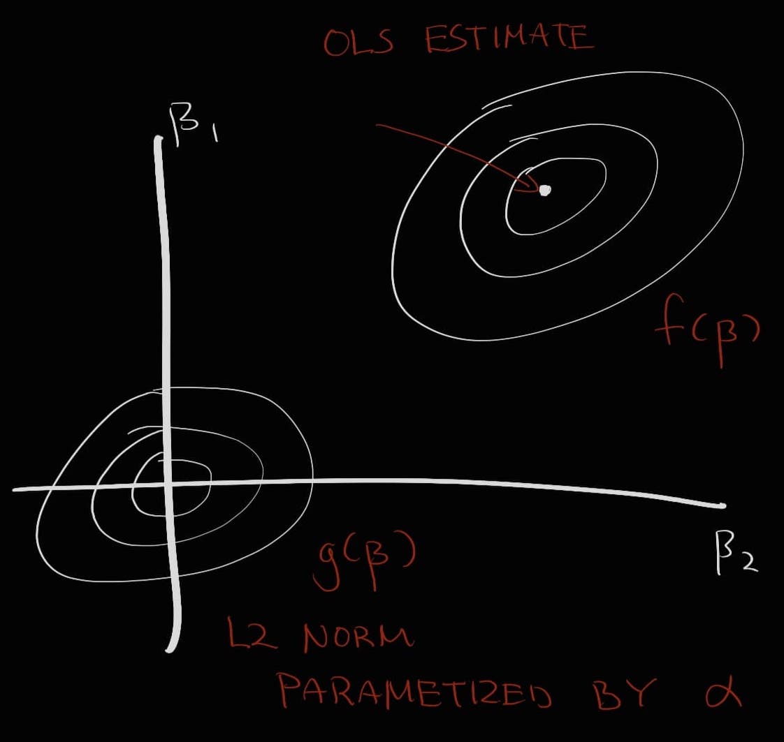
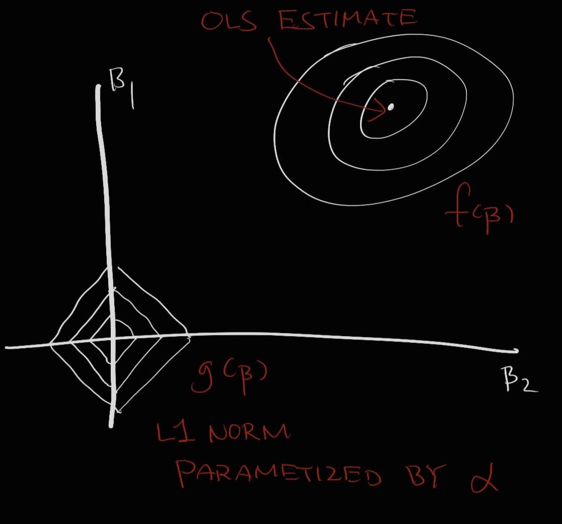
Geometric interpretation of Ridge and Lasso regression

Typically, the estimate of the ordinary least squares (OLS) regression and the Ridge or Lasso regression are plotted as a function of the model weights in order to explain L1 and L2 regularization.

Consider the following: there exists a function f that describes the non-penalized form to a linear model (i.e., the MSE). The minimum of this function describes the solution to the linear regression. This function is represented as an elliptical contour. As these contours expand, the residual sum of squares (RSS) increases. Now say there is the penalized form of this model described by another function g. This g as a function of (i.e., the model weights) equals to either the L1 norm of the sum of weights (Lasso) or the L2 norm of the sum of squared weights (Ridge) multiplied by the parameter . This function is drawn in the shape of a diamond (Lasso) or a ball (Ridge). At higher values of - that is, the harsher penalty term - the contour plot described by g gets narrower and narrower. The point at which the two contours f and g meet is the regularized solution to the model.

Evidently, there exists a balance between increasing the RSS or decreasing the penalty. If we decrease the penalty more and more, the two contours will meet closer to the center of the contour f - the non-penalized solution. At the extreme level, setting the penalty to zero will lead to non-penalized OLS. If we increase the penalty on the other hand, eventually the solution will reach zero.

Furthermore, due to the shape of the contour plot described by the L1 norm, it is such that the intersection between f and g is likely to occur at the corners of the diamond - where either \(\beta_{1}\) or \(\beta_{2}\) is equal to zero. This leads to a sparse solution where a feature is set to zero, as described earlier.