Visualizing the gradient descent in R
The general idea of the gradient descent is to iteratively tweak parameters with the goal of minimizing a loss function. In the case of a linear regression model, the loss function is simply described by the mean-squared-error (MSE) - which is essentially the sum of squared residuals. The parameters to tweak in such a model would be the slope and the intercept of the regression line.
MSE is described by a quadratic function; this means that the further away you are from the minimum point, the steeper the slope. The concept of the gradient descent is to tweak the tangent line (which is described by the slope and the intercept) by some value (also known as the 'learning rate') until we've hit the inflection point of the parabola, that is, the minimum value of the loss function. A classic visualizer for the above problem is the ball rolling down the parabolic curve until it settles at the foot of the hill.
The gradient descent algorithm requires the function to be both differentiable and convex. The MSE function satisfies both criteria. The mathematical derivation of the gradient descent is described below:
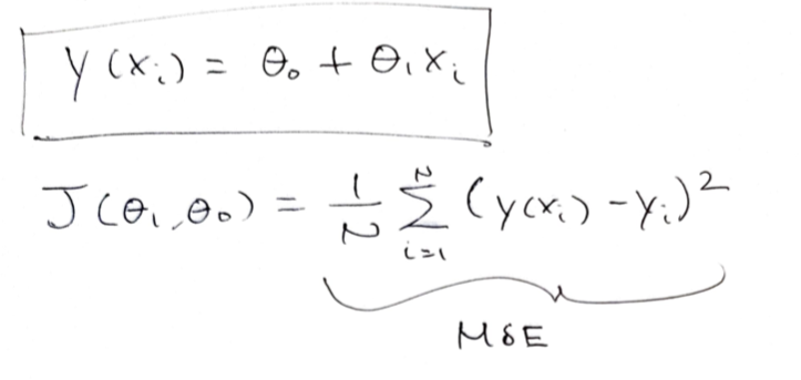
The response variable \(y\) is a function of some predictor \(x_{i}\). \(\theta_i\) describes the slope and \(\theta_0\) describes the y-intercept. The loss function is the MSE.
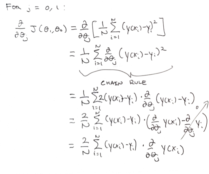
Firstly, the partial derivatives with respect to the slope and the intercept must be solved. The general solution for the partial derivative w.r.t both the slope and the intercept is shown above.
The result so far is the sum of residuals and a partial derivative term. The partial derivative term itself can be solved trivially for both the slope and the intercept as follows:
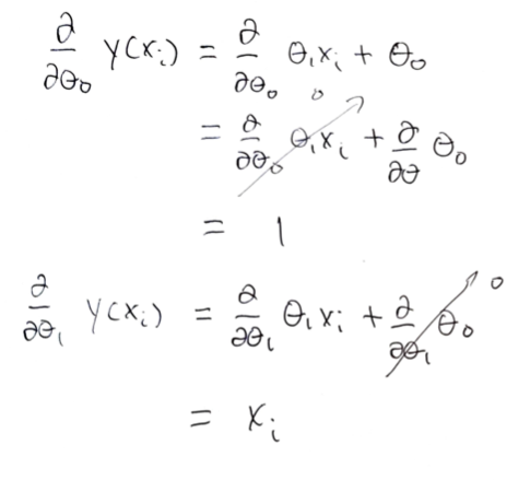
Substituting the values for the respective partial derivatives, the equation we arrive at is:
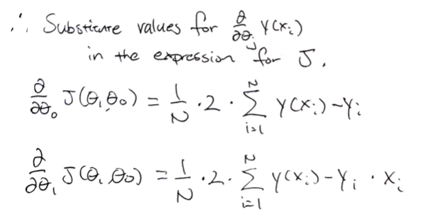
In other words, the derivative w.r.t the intercept term is simply the sum of residuals multiplied by a constant. The derivative w.r.t the slope term is the same, with an extra \(x_i\) term. The partial derivatives then must be multiplied by the learning rate (i.e., the increment to which the parameters will be changed) to arrive at new values for the slope and the intercept. Once the calculated loss for the new set of parameters converge, the iterative process can terminate.
The gradient descent algorithm applied to a linear regression model can be demonstrated in R as follows:
library(tidyverse)
set.seed(1000)

theta_0 <- 5
theta_1 <- 2
n_obs <- 500
x <- rnorm(n_obs)

y <- theta_1*x + theta_0 + rnorm(n_obs, 0, 3)

rm(theta_0, theta_1)

data <- tibble(x = x, y = y)

ggplot(data, aes(x = x, y = y)) + geom_point(size = 2) + theme_bw() + labs(title = 'Simulated Data')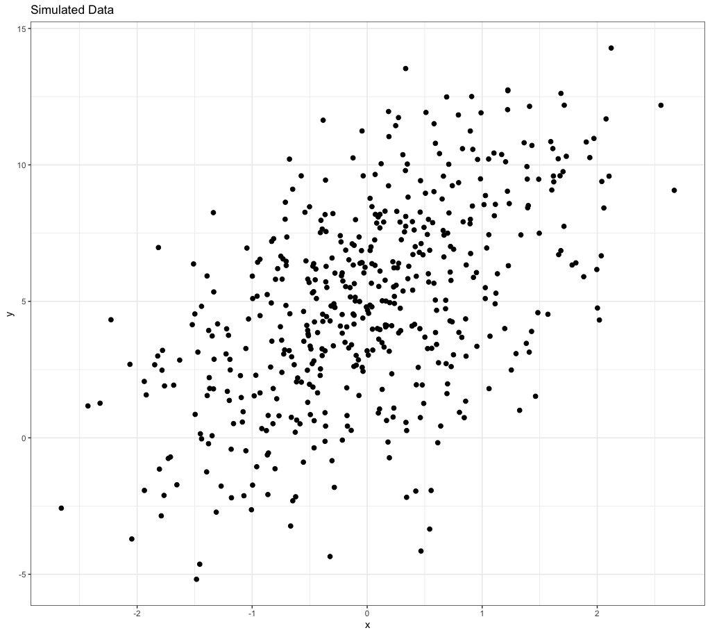
ols_fit <- lm(y ~ x, data = data)
summary(ols_fit)
ols_fit$coefficients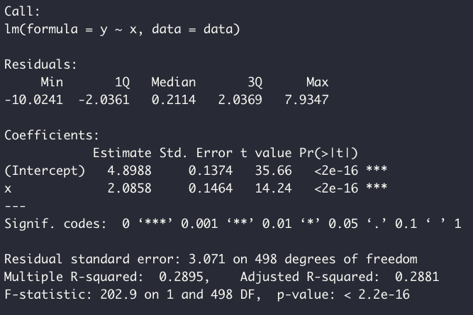

Above, we've created synthetic data and fit it to a linear model. The coefficients for the model (i.e., the slope and the intercept) are printed above. We can now write a function to calculate the loss:
cost_function <- function(theta_0, theta_1, x, y){
  pred <- theta_1*x + theta_0
  res_sq <- (y - pred)^2
  res_ss <- sum(res_sq)
  return(mean(res_ss))
}

cost_function(theta_0 = ols_fit$coefficients[1][[1]],
         theta_1 = ols_fit$coefficients[2][[1]],
         x = data$x, y = data$y)

sum(resid(ols_fit)^2)

As above, the calculated loss corresponds to the MSE from the linear model.
The gradient descent function can be written as follows. Note that the delta_theta_0 and the delta_theta_1 correspond to the derived expressions for the partial derivatives earlier. We then write a subsequent function to apply the algorithm after defining our learning rate (alpha) and the number of times we will iterate through the algorithm.
gradient_desc <- function(theta_0, theta_1, x, y){
  N = length(x)
  pred <- theta_1*x + theta_0
  res <- y - pred
  delta_theta_0 <- (2/N)*sum(res)
  delta_theta_1 <- (2/N)*sum(res*x)
  return(c(delta_theta_0, delta_theta_1))
}

alpha <- 0.1
iter <- 100

minimize_function <- function(theta_0, theta_1, x, y, alpha){
  gd <- gradient_desc(theta_0, theta_1, x, y)
  d_theta_0 <- gd[1] * alpha
  d_theta_1 <- gd[2] * alpha
  new_theta_0 <- theta_0 + d_theta_0
  new_theta_1 <- theta_1 + d_theta_1
  return(c(new_theta_0, new_theta_1))
}
The gradient descent algorithm needs a set of random initial values (i.e., initialization of the model). We will start at (0, 0) - that is, slope of 0 and intercept of 0 then progressively iterate through the gradient descent algorithm and see if we approach the coefficient values we got from the linear model earlier.
res <- list()
res[[1]] <- c(0, 0)

for (i in 2:iter){
  res[[i]] <- minimize_function(
    res[[i-1]][1], res[[i-1]][2], data$x, data$y, alpha
  )
}

res <- lapply(res, function(x) as.data.frame(t(x))) %>% bind_rows()
colnames(res) <- c('theta0', 'theta1')

loss <- res %>% as_tibble() %>% rowwise() %>%
  summarise(mse = cost_function(theta0, theta1, data$x, data$y))

res <- res %>% bind_cols(loss) %>%
  mutate(iteration = seq(1, 100)) %>% as_tibble()

res %>% glimpse()
From the data frame above, we can see that the values for the slope and the intercept are both approaching the values we got from the linear model (i.e., 4.898 and 2.085, respectively). The loss (MSE) also decreaes over iterations, as we expected. We can plot the loss versus the number of iterations to show this.
ggplot(res, aes(x = iteration, y = mse)) + geom_point(size = 2) +
theme_classic() + geom_line(aes(group = 1)) 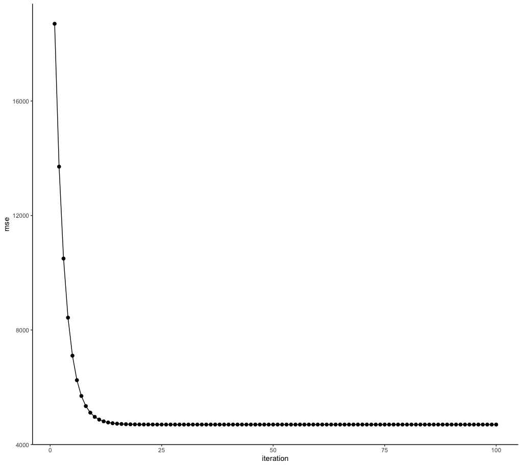
It looks like we didn't need anywhere near 100 iterations to converge at the minimum value.
Below, the iterative nature of the gradient descent is shown - the regression line at each iteration is plotted in red across our synthetic data. The blue line is the regression line at iteration = 1; a line with slope of zero and intercept of zero. Over time, the regression line is optimized until the green line is drawn - the regression line at iteration = 100, which describes our line of best fit.
ggplot(data, aes(x = x, y = y)) +
  geom_point(size = 2) +
  geom_abline(aes(intercept = theta0, slope = theta1),
              data = res, size = 0.5, color = 'red') +
  theme_classic() +
  geom_abline(aes(intercept = theta0, slope = theta1),
              data = res %>% slice_head(), size = 0.5, color = 'blue') +
  geom_abline(aes(intercept = theta0, slope = theta1),
              data = res %>% slice_tail(), size = 0.5, color = 'green')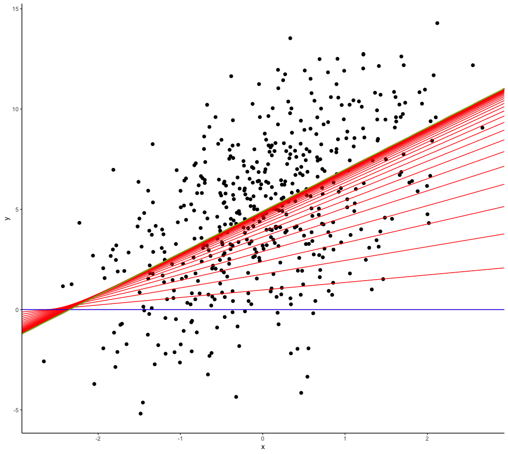
In summary, the gradient descent is an iterative algorithm which seeks the minimum value for a differentiable, convex function. This can be used to find the optimal values for a set of parameters by minimizing the model loss, as in the case of the linear regression model shown above. The formula for the gradient descent can be derived by using a set of partial derivatives with respect to each model parameter and applying a fixed learning rate.