Streamlining machine learning projects with caret
A typical predictive learning workflow consists of five main facets. These are:
- data splitting
- data pre-processing
- feature selection
- model training and tuning
- variable importance estimation
The caret package in R streamlines this process by offering a set of function that executes the above and more (e.g., multiple model comparisons, sub-sampling, etc.). The R object containing the trained model from caret can also be used by other packages such as MLeval and MLmetrics, which digs deeper into predictive model evaluations.
Say we were solely concerned with building an optimal predictive model for a Kaggle project. Where do we start? Here, I've downloaded a toy dataset from Kaggle (https://www.kaggle.com/kkhandekar/all-datasets-for-practicing-ml) which contains properties of different wine (the predictors, x) and a wine quality rating (the class - also known as the ground truth, Y). The goal will be to build a predictive model based on this data using caret.
In general, it's a good idea to convert the class column - here it's named 'quality' and it is an integer value - as a factor.
library(tidyverse)
df <- read_delim('Class_Winequality.csv', delim = ';')
df <- df %>% mutate(quality = factor(quality)) %>% relocate(quality)
summary(df %>% select(-quality))
Quick summary of the predictor variable shows the following:
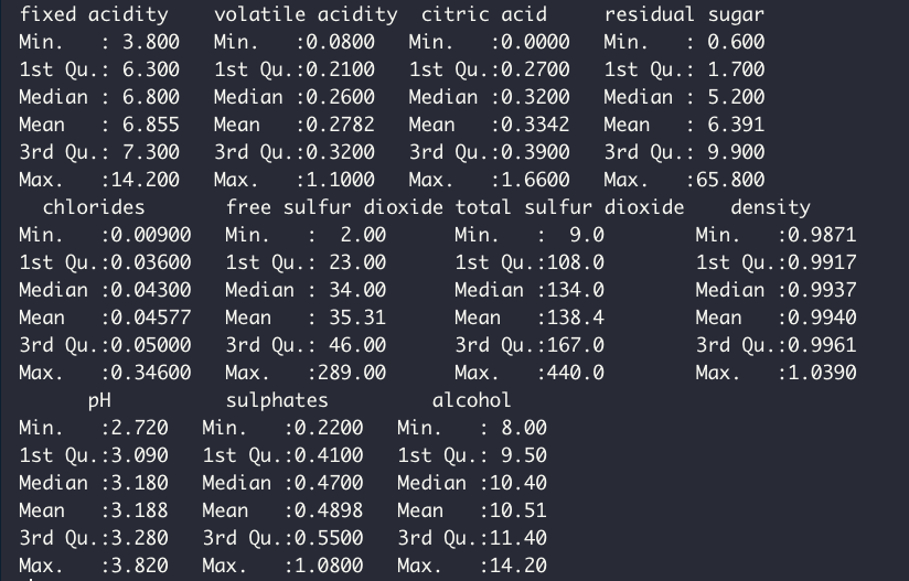
It's apparent that our set of predictors are heterogeneous in terms of their ranges. Usually, it's a good rule of thumb to have small predictor values, possibly centered and scaled to have a mean of zero and standard deviation of 1. The exact nuance of whether a predictor variable needs pre-processing depends on the analysis and problem at hand. Here, without pre-processing, this is what our predictors look like in terms of distribution:
df2 <- df %>% pivot_longer(-quality, names_to = 'Property', values_to = 'Values')

ggplot(df2, aes(x = quality, y = Values)) + geom_boxplot(aes(fill = quality), alpha = .4) + facet_wrap(~Property, scales = 'free') + theme_classic() + theme(legend.position = 'none')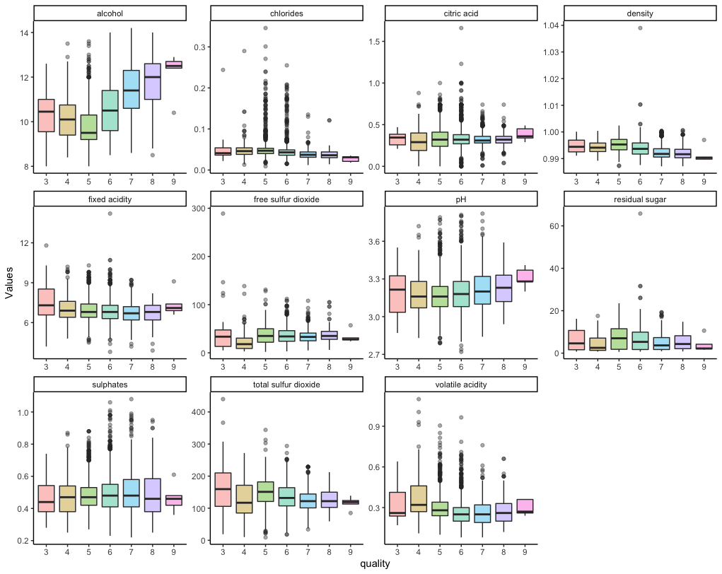
Later, I will pre-process the data and compare the distribution.
First, as caret does not like the class variable to start with a number, I am changing the variable values slightly to have a 'Class_' prefix. The data is then split into 80/20 partitions for model training.
library(caret)
set.seed(12345)

df <- df %>% mutate(quality = factor(str_c('Class_', quality)))

trainIdx <- createDataPartition(df$quality, p = .8,
                                  list = FALSE,
                                  times = 1)

df_train <- df[ trainIdx,]
df_test  <- df[-trainIdx,]
dim(df_train)
dim(df_test)
Now I pre-process the training and testing data. Here I define the pre-processing method as 'center' and 'scale' to do the following:
- Center: subtract the data by the overall mean
- Scale: divide the centered data by the overall standard deviation
Note that I can pass every column into the preProcess function, as it will ignore columns which are factors. Thus we don't have to worry about whether it will mess with our class column values.
preProcValues <- preProcess(df_train, method = c('center', 'scale'))
preProcValues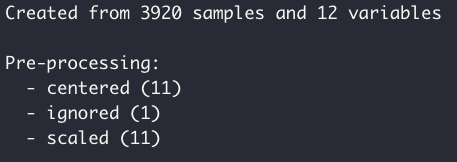
Using the preProcess object, I transform the training and testing data:
df_train <- predict(preProcValues, df_train)
df_test <- predict(preProcValues, df_test)
Now when I check the distribution of the predictors, the data are clearly centered around zero.
summary(df_train %>% select(-quality))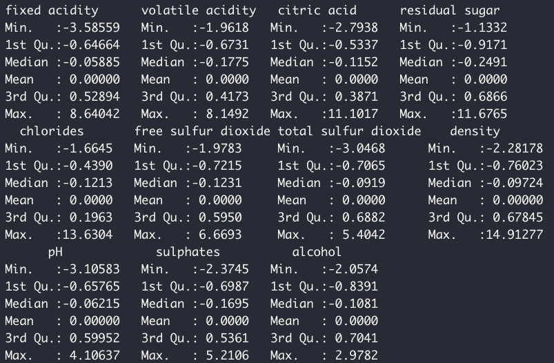
Training a model with the pre-processed data is simple: here, my model of choice is a Random Forest classifier, which is specified by the 'ranger' method within the train function. For the re-sampling of the training data, I am using a 5-fold cross validation. Note here I can specify different methods of re-sampling, such as out-of-bag or repeated k-fold.
tr <- trainControl(method = 'cv', number = 5, classProbs = TRUE)

model <- train(quality ~., data = df_train, method = 'ranger', importance = 'impurity', trControl = tr)

model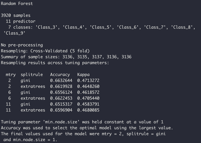
Caret automatically runs model tuning to find the optimal set of hyperparameters. We can also directly specify a range of hyperparameters we'd like to test, which is shown later.
model$bestTune
The tuned model is tested using the test data set, which was unseen by the model during the training and tuning process. The confusion matrix shows the proportion of corrected classified samples per class.
pred <- predict(model, df_test)

confusionMatrix(pred, df_test$quality)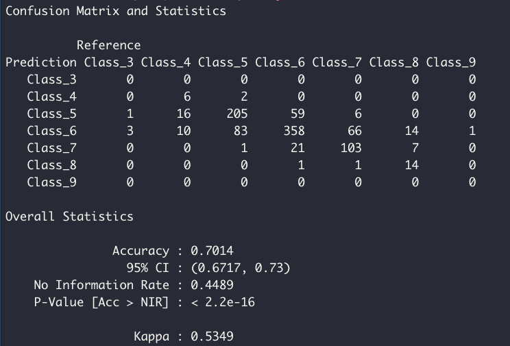
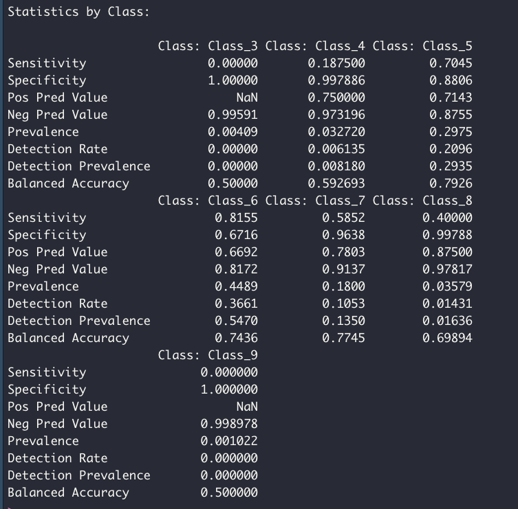
Extracting variable importance from the trained model is also straightforward:
df_imp <- varImp(model)$importance %>% rownames_to_column(var = 'Var') %>%
  as_tibble() %>% arrange(desc(Overall))

ggplot(df_imp, aes(x = reorder(Var, Overall), y = Overall)) +
  geom_point(stat = 'identity', color = 'red') +
  geom_segment(aes(x = reorder(Var, Overall),
                   xend = reorder(Var, Overall),
                   y = 0,
                   yend = Overall)) +
  theme_classic() + coord_flip() + xlab('') + ylab('Var. Imp.')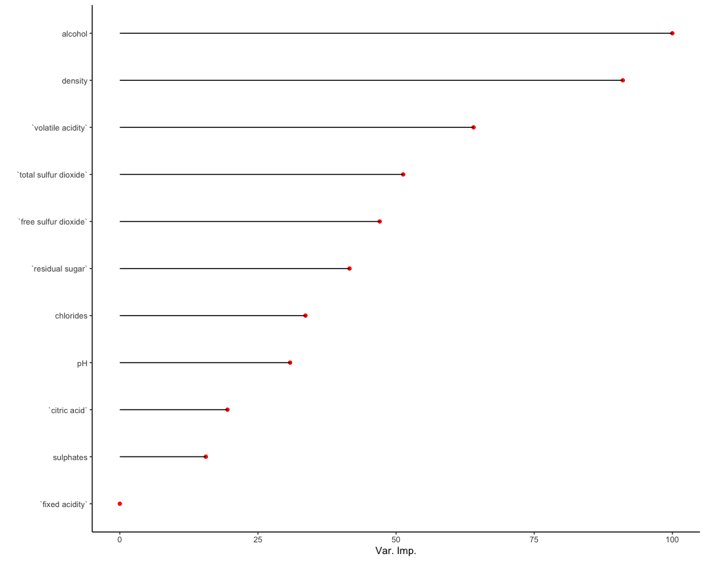
Note the default values for variable importance are normalized such that the top variable is set to a value of 100. This behavior can be turned off by setting 'scale = FALSE' within the varImp function. As specified during the model training process, the variable importance here is defined by a decrease in Gini impurity following permutation of a given predictor variable x.
In cases where our data set contains an enormous amount of predictor variables, feature selection may be considered. In our case, since we only had a dozen variables this was not an issue. Regardless, here I run a feature selection algorithm to demonstrate the central concept. Feature selection essentially boils down to selecting the top n predictor variables sorted by some measure of importance or value. This can involve using wrapper functions as in the case of recursive feature selection - which essentially fits a model such as the random forest and ranks variables by variable importance - as well as dimensionality reduction techniques such as PCA. Feature selection can improve the analysis by reducing the overall training time and computational load, reducing the risk of over-fitting, and improving overall model accuracy.
Two of the simplest feature selection methods caret offers are anovaScores and gamScores. As the name implies, anovaScores fits a simple OLS model between the predictors and the class variable. Generalized additive models (GAMs) are used by gamScores instead. Both methods return a p-value indicating the likelihood of a relationship between a given predictor
x and the class variable Y. Here, I define a function using anovaScores and run feature selection on our training data.
fit_anova <- function(x, y) {
    anova_res <- apply(x, 2, function(f) {anovaScores(f, y)})
    return(anova_res)
}

anova_res <- fit_anova(x = select(df_train, -quality), y = df_train$quality)

anova_res <- as.data.frame(anova_res)

anova_res <- anova_res %>% rownames_to_column(var = 'Var') %>% as_tibble() %>% rename(anova_pVal = anova_res) %>% arrange(anova_res)


ggplot(anova_res, aes(x = reorder(Var, -anova_pVal), y = -anova_pVal)) +
  geom_point(stat = 'identity', color = 'red') +
  geom_segment(aes(x = reorder(Var, -anova_pVal),
                   xend = reorder(Var, -anova_pVal),
                   y = 0,
                   yend = -anova_pVal)) +
  theme_classic() + coord_flip() + xlab('') + ylab('ANOVA p-Val.')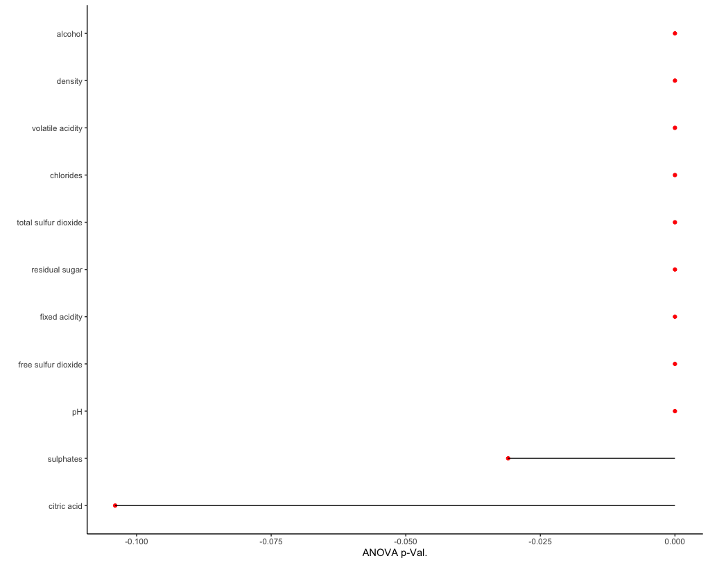
As seen, the top predictors from feature selection reflect the variable importance results from our predictive model. This is unsurprising, as our data is relatively simple and low dimensional.
Caret also offers comparison of multiple predictive models. Here, using the same training set, I define three additional models:
- support vector machine using radial basis function ('svmRadial')
- gradient boosting machine ('gbm')
- k-nearest neighbors ('knn')
Note that for each model training, caret tunes each model's respective hyperparameters to arrive at a final model (e.g., 'k' for the k-nearest neighbor model, 'C' (cost) for the support vector machine model).
Collating the three new models with the previous random forest model is done using the 'resamples' function.
model2 <- train(quality ~., data = df_train, method = 'svmRadial', trControl = tr)

model3 <- train(quality ~., data = df_train, method = 'gbm', trControl = tr, verbose = FALSE)

model4 <- train(quality ~., data = df_train, method = 'knn', trControl = tr)

comps <- resamples(list(RF = model, SVM = model2, GBM = model3, KNN = model4))
The model performances are summarized as such:
summary(comps)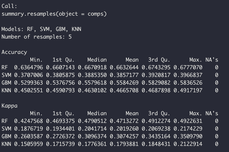
This is visualized by the following:
dotplot(comps)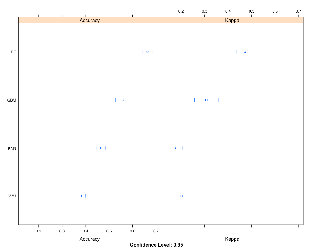
Finally, in order to fine-tune the model parameters ourselves, I can provide a range for each hyperparameter myself. Providing this information to the model training step is also straightforward:
ranger_grid <- expand.grid(mtry = c(2, 4, 8, 10), splitrule = c("gini", "extratrees"), min.node.size = c(1, 3, 5))

model5 <- train(quality ~., data = df_train, method = 'ranger', importance = 'impurity', trControl = tr, tuneGrid = ranger_grid)

model5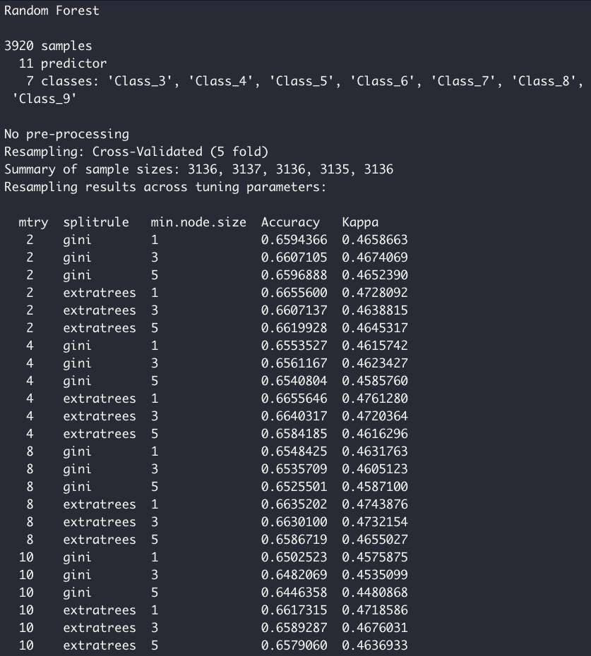
In summary, caret allows an easy access to a streamlined workflow. Despite the simple nature of automation, however, user must take necessary caution at each step to guide each piece of input and output. Feature engineering, for instance, is a vital chunk of data preparation and a priori knowledge of input data can guide model preparation. Real life data often requires imputation, which can have a great impact on model interpretation as well as performance. Considerations in correlating variables and co-linearity must also be considered. Regardless, the five aforementioned facets of every machine learning problem remains vital and at the forefront of a typical workflow.