Precision, recall, and decision functions in classifier models

The Problem of Unbalanced Data

First, generate a synthetic dataset with unbalanced classes (labels):

import numpy as np
from sklearn.datasets import make_classification

x, y = make_classification(n_samples=10000, n_features=2, n_redundant=0, n_clusters_per_class=1, weights=[0.95], random_state=42)
                           
label, counts = np.unique(y, return_counts=True)

print(np.asarray((label, counts)).T)

As you can see, only around 5% of the target labels are encoded as '1', while the rest are '0's. Now we naively fit a classifier model to this data as-is:

For this exercise I am using a linear support vector machine with a 30/70 training-testing split.

from sklearn.model_selection import train_test_split
from sklearn.svm import SVC

x_train, x_test, y_train, y_test = train_test_split(x, y, test_size=0.3, random_state = 42)

svm_model = SVC(kernel = 'linear', C = 1)
svm_model.fit(x_train, y_train)
y_pred = svm_model.predict(x_test)

Now evaluate the model on the test data using a plain accuracy metric as well as a cross-validation with 10-folds:

from sklearn.model_selection import cross_val_score
from sklearn.metrics import accuracy_score

print('Accuracy:', accuracy_score(y_test, y_pred))
scores = cross_val_score(svm_model, x, y, cv = 10)
print("K-fold cross validation accuracy: %0.2f (+/- %0.2f)" % (scores.mean(), scores.std() * 2))

99% model accuracy indicates this model is exceptional at predicting the correct class. But what if we had a 'model' that was so incompetent that it predicted nothing but 0s all the time - regardless of predictor variables?

y_pred_dummymodel = np.tile(0, 3000)
print('Accuracy:', accuracy_score(y_test, y_pred_dummymodel))

The completely incompetent model achieves 94%, which rightfully exposes the faults of our ways. This is exactly the reason why we should consider something like SMOTE to balance our data. But what if we look at more robust ways to evaluate our model?

Precision and Recall

The precision evaluates the percentage of correct classifications out of all positive hits. A model that results in zero false positive cases has a precision of 1.0.

The recall evaluates the percentage of positive hits which were identified correctly. A model that results in zero false negative cases has a recall of 1.0.

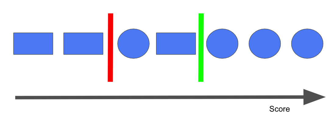
These two metrics coexist in a push-and-pull relationship. Consider the following: we are trying to build a model that distinguishes between circles and squares. Let's say this model has some sort of an internal threshold score such that when score > threshold score, it classifies the object as the positive class (in this case, let's assign the positive class as a circle). If this hypothetical threshold score is denoted by the green vertical bar, the model predicts everything on the right side of the bar as a circle and everything else, a square. Our precision score would be 3/(3+0) = 1.0 and our recall score would be 3/(3+1) = 0.75. If the threshold score was the red bar instead, our precision would be 4/(4+1) = 0.8 and recall 4/(4+0) = 1.0. So at an attempt to increase one, we've decreased the other score. This behaviour is as known as the precision/recall trade-off.

from sklearn.metrics import precision_recall_curve
from sklearn.model_selection import cross_val_predict

y_scores = cross_val_predict(svm_model, x_train, y_train, cv=3,
                             method="decision_function")
precision, recall, thresholds = precision_recall_curve(y_train, y_scores)

import matplotlib.pyplot as plt

plt.style.use('fivethirtyeight')
plt.plot(thresholds, precision[:-1], "b--")
plt.plot(thresholds, recall[:-1], "g-")
plt.show()

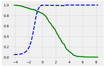
Plotting precision and recall across decision thresholds reflects this tug-of-war behavior. The ideal situation then, is to pick a decision threshold which maximizes one before a steep drop-off in the other.

The F1 score is a metric which consolidates both precision and recall into a single value. The exact derivation of this score is not shown here, but it is essentially a harmonic mean of the precision and recall scores, which gives higher weights to low values.

from sklearn.metrics import f1_score

f1_score(y_test, y_pred)

Decision Functions and Loss Functions

The hypothetical 'decision threshold' above is not hypothetical at all. In fact, the idea of the threshold is based on a concept as known as the decision function which is loosely defined as a function that outputs a decision based on input data. In classification problems, this decision is is a prediction into a class. This function shouldn't be confused with the loss function, which is taken into account by the decision function and describes an estimated cost associated with each decision. The most obvious loss function is the mean-squared-error in regression problems, or cross-entropy in binary classification models.

In linear support vector machines, the decision boundary is defined as a line (or a 'hyperplane') which maximizes the distance from linearly separable classes (i.e., data points belonging to two distinct classes). The support vector machine model then reduces to an optimization problem which attempts to maximize the margins from the decision boundary (i.e., the hyperplane). This is summarized by a hinge loss function, which attempts to minimize the error associated with the margin.

This hinge loss function can then be optimized by methods such as the gradient descent. In Scikit-Learn, we can do this by calling the stochastic gradient descent classifier:

from sklearn.linear_model import SGDClassifier

SGD_model = SGDClassifier(loss="hinge", penalty="l2", max_iter=20)
SGD_model.fit(x_train, y_train)
y_pred2 = SGD_model.predict(x_test)
f1_score(y_test, y_pred2)

Above code fits a linear support vector machine on our previous training data with L2 regularization. We can inspect our decision function as well:

x1 = x_test[0]
x1 = x1.reshape(1, -1)

SGD_model.decision_function(x1)

Since this is a binary classification problem, the output of decision function is simple. The output tells us which side of the hyperplane the data point is on. Based on this decision function output, the data point is classified as one label or the other.

ROC Curves

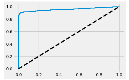
Finally, the concept of the decision threshold, precision, and recall leads to the widely used ROC curves. ROC curves plot recall (true positive rate) versus the false posiive rate. Each metric is plotted across a range of decision thresholds.

from sklearn.metrics import roc_curve

fpr, tpr, thresholds = roc_curve(y_train, y_scores)

plt.plot(fpr, tpr, linewidth=3)
plt.plot([0, 1], [0, 1], 'k--')
plt.show()

The tpr = fpr diagonal line indicates a completely random classifier. An effective model's ROC curve hugs the upper left corner - which can be quantified by the area under the curve.

from sklearn.metrics import roc_auc_score

roc_auc_score(y_train, y_scores)

Concluding Remarks

In summary:

• Unbalanced datasets require special care in model assessment

• Metrics such as precision, recall, and F1 score provide a more robust way to evaluate classifier model

• The decision threshold and associated decision functions affect the precision/recall trade-off

• Models such as support vector machines are optimized using a loss function, which in turn is used by the decision function

• ROC curves reflect the change in true- and false-positive rates across a range of decision thresholds

Code + Jupyter notebook used for this post is available on my GitHub Repo.