ANOVA and linear regression: same but different
I preface this post with a bit of a digression. The other day I was looking at ways to perform feature selection prior to running a classifier model and the R package caret offered me two ways to do it: generalized additive models (i.e., GAMs) and ANOVA. As you may be aware, GAMs are a strategy to perform non-linear predictor vs. response modeling using splines. ANOVA, on the other hand, may be the very first thing we learn in an introductory stats course. It's analysis of variance and tests whether there is an underlying effect causing variance among groups of means. In other words, it's an extended T-test across multiple groups.
However, the more we read about ANOVAs, the more we see parallels between them and simple linear regression. In fact, many stats packages in R and Python use the terms ANOVA and OLS (ordinary least squares) to essentially say the same thing. Why did we learn about them in separate contexts in our stats courses then? Are they the same?
The short answer is yes - almost. The long answers can be found by digging through Stats Exchange forums and scientific publications. Here is my best explanation, presented in a more digestible way.
Linear regression
Linear regression estimates how much a response variable Y changes when predictor variable X changes by a certain amount. This relationship is predicted by using a linear relationship:
\(Y = \beta_0 + X\beta_1 + \epsilon\)
Here, X is assumed to be a numeric vector of constant variables. \(\beta_0\) denotes the intercept of the regression line - predicted value for Y when X = 0. \(\beta_1\) is the coefficient for X, also called the parameter estimate or the weight for predictor X. \(\epsilon\) is the error term and is assumed to be normally distributed, i.e., \(\epsilon \in N \sim (0, \sigma^2)\).
In multiple linear regression (i.e., more than one predictor variable), we can simply add more \(X_i\) terms with their own coefficients \(\beta_i\) for \(i \in R\).
In R, we can fit a linear model as such: using my favorite toy dataset mtcars.
require(tidyverse)
df <- mtcars %>% select(c(mpg, disp, hp, drat, wt, qseq))
lm_model <- lm(mpg ~., data = df)
In Python, we can use the scikit-learn package (statsmodel package works too):
from sklearn.linear_model import LinearRegression

predictors = ['disp', 'hp', 'drat', 'wt', 'qseq']
outcome = 'mpg'

model = LinearRegression()
model.fit(mtcars[predictors], mtcars[outcome])
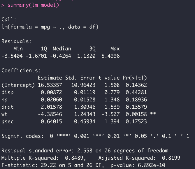
We can view the individual coefficients for each of the predictor variables and the associated standard errors and p-values by calling:
summary(lm_model)
ANOVA
As mentioned earlier, ANOVA is testing the effect of a given treatment across many groups. We can think of this as a comparison between the variance due to treatment versus a random variance due to chance. In other words, the total variability across many groups can be decomposed into:
\(Y_{ij} - \overline{Y}.. = \overline{Y}_i. - \overline{Y}.. + Y_{ij} - \overline{Y}_i.\)
The left-hand side denotes the total deviation. The first term on the right-hand side denotes the deviation of estimated group mean around overall mean. The second term denotes the deviation around group mean, AKA simmply the error \(\epsilon_{ij}\).
The parametization of ANOVA leads to the effects model equation:
\(Y_{ij} = \mu + \tau_{i} + \epsilon_{ij}\)
\(\mu\) denotes the grand population mean, \(\tau_{i}\) denotes the deviations from the grand mean due to group effects, and \(\epsilon_{ij}\) denote the error terms. In ANOVA, the null hypothesis states group effects are all zero and the above equation is reduced down to:
\(Y_{ij} = \mu + \epsilon_{ij}\)
Where the null hypothesis can be stated as:
\(H_{0} = \tau_{1} = ... = \tau_{n} = 0\)
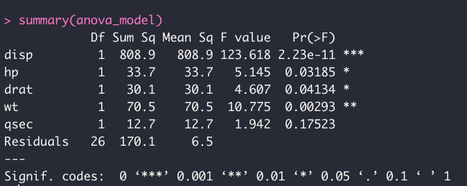
Of course, then it must be that the alternate hypothesis states group effects are nonzero. In practical terms, the ANOVA employs an F-statistic, which is defined as the ratio between the mean squares (MS) of between-groups and mean squares of the error term. Note mean squares are just the sum of squares standardized by the degrees of freedom.
The ANOVA implementation is also simple on R:
anova_model <- aov(mpg ~., data = df)

summary(anova_model)
The equivalent test in Python is done with statsmodels:
import statsmodels.formula.api as sm
anova_model = sm.ols(formula = 'mpg ~ disp + hp + drat + wt + qseq', data = df)
print(anova_model.summary())
Putting them together
Above Python code should already key you in the similarities between linear regression and ANOVA, as well as the effects model equation. Indeede, the effects model equation is analogous to the linear regression model equation. For an example with two predictor variables:
ANOVA:
\(Y_{ij} = \mu + \tau_{1}\beta_{1} + \tau_{2}\beta_{2} + \epsilon_{ij}\)
OLS:
\(Y_{ij} = \beta_{0} + X{1}\beta_{1} + X{2}\beta_{2} + \epsilon_{ij}\)
The first term in each equation's right hand side equates to the grand mean with no contribution from individual group means (ANOVA) and the y-intercept of the regression line (OLS) - which, in fact, is not affected by the individual predictor terms. In other words, in both analogous cases, this term is a constant.
\(\tau_{1}\beta_{1}\) and \(\tau_{2}\beta_{2}\) terms in ANOVA represent the deviations from \(\mu\) due to predictors \(X_{1}\) and \(X_{2}\) respectively, with the \(\beta\) terms denoting the slopes of the covariates for each group.
\(X{1}\beta_{1}\) and \(X{2}\beta_{2}\) terms in linear regression represent the deviations from the intercept weighted by \(\beta\), due to each continuous variable \(X_{1}\) and \(X_{2}\). Then it must be, that ANOVA and OLS do indeed represent the same concept, except in ANOVA we are dealing with groups rather than continuous variables. These groups - whether they are treatment groups in a drug study or a age bracket group in a consumer analysis - must then be represented by dummy variables in a typical regression analysis. For example, groups belonging to treatment group A can be zeroes, and the other group can be 1s.
The take-home message at this point should be that ANOVA essentially boils down to a linear regression of dummy encoded variables.
Driving home this point, going back to the actual code and the mtcars dataset - if we extract the coefficients of each model, we see that they are actually equal:
lm_model$coefficients
anova_model$coeffcients
Alternative look: matrix operations
Another way to visualize the parallels between ANOVA and OLS is by inspecting the model matrices. In the case of the ANOVA, the matrix projection can be shown as:
\[\left[\begin{array} {rrr} Y_1 \\ Y_2 \\ Y_3 \\ \dots \\ \dots \\ Y_n \end{array}\right] = \]
\[ \begin{pmatrix} 1 & 0 & 0\\ 1 & 0 & 0\\ \dots & \dots & \dots\\ \dots & \dots & \dots\\ 0 & 1 & 0\\ 0 & 1 & 0\\ \dots & \dots & \dots\\ \dots & \dots & \dots\\ 0 & 0 & 1\\ 0 & 0 & 1\\ \end{pmatrix} \left[\begin{array} {rrr} \tau_1 \\ \tau_2\\ \tau_3\\ \end{array}\right] + \left[\begin{array} {rrr} \epsilon_1\\ \epsilon_2\\ \epsilon_3\\ \dots\\ \dots\\ \epsilon_n\\ \end{array}\right] \]
Above describes a one-way ANOVA model matrix with three groups, again, summarised as \(Y_{ij} = \mu + \tau_{i} + \epsilon_{ij}\) where \(\tau\) is the mean at each group. The model matrix for linear regression is straightforward and is shown below:
\[\left[\begin{array} {rrr} Y_1 \\ Y_2 \\ Y_3 \\ \dots \\ \dots \\ Y_n \end{array}\right] = \]
\[ \begin{pmatrix} 1 & x_{12} & x_{13}\\ 1 & x_{22} & x_{23}\\ 1 & x_{32} & x_{33}\\ \dots & \dots & \dots\\ \dots & \dots & \dots\\ 1 & x_{n2} & x_{n3} \end{pmatrix} \left[\begin{array} {rrr} \beta_1 \\ \beta_2\\ \beta_3\\ \end{array}\right]+ \left[\begin{array} {rrr} \epsilon_1\\ \epsilon_2\\ \epsilon_3\\ \dots\\ \dots\\ \epsilon_n\\ \end{array}\right] \]
Above can be represented as \(Y = \beta_0 + X_{i1}\beta_1 + X_{i2}\beta_2 + \epsilon_{i}\) with the y-intercept \(\beta_{0}\) and two slopes for each contiuous variable.
Here, again it is clear that ANOVA is analogous to OLS in such a way that variables are dummy encoded and each predictor term represents a group mean rather than a continuous variable.