Random Forests in R: bootstrapping and aggregating
In predictive models, decision trees produce a set of rules to classify or predict a given outcome. As their names suggest, decision trees employ a series of branches to successively partition data. In brief, this method is called 'recursive partitioning' wherein each split references a specific value of a variable and divide the data whether the record is above or below that value. At each branching point of the tree, the model picks the split value that minimizes the outcome impurity within each sub-parition.
An 'ensemble' method forms predictions by using a collection of models. Ensemble of tree models make up the random forest (RF) algorithm, which use two techniques:
bootstrapping of records to form a bootstrap sample (i.e., sampling with replacement)
random sampling of predictor variables to create sub-paritions
Essentially, RF models use the predictive power of an ensemble of many decision trees, where each tree use a random subset of predictor variables and a bootstrap sample.
In R, RF model can be implemented using the randomForest package. Here, a dataset of iris flowers from Kaggle (https://www.kaggle.com/souravbhattacharya10/irisdataset) is used to predict iris species. The features include petal length, petal width, sepal length, and sepal width.
install.packages('randomForest')
library(randomForest)
library(tidyverse)

df <- read_csv('Iris.csv')
head(df)
summary(df)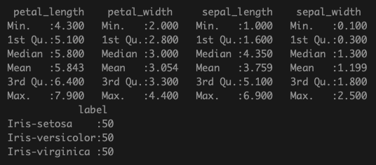
Splitting the dataset into training and validation split can be done with base R. Here I use a 80/20 split using sample function to randomly divide the data.
set.seed(42)
df$label <- factor(df$label)
train_subset <- sample(nrow(df), 0.8*nrow(df), replace=FALSE)
df_train <- df[train_subset,]
df_val <- df[-train_subset,]
There are a number of parameters to consider when fitting an RF model.
Number of trees. In randomForest function in R, this is ntree. Default is 500. This parameter denotes the total number of trees to be fit in the ensemble.
Number of picked variables during the bootstrap-aggregation process. In randomForest function, this is mtry. Default is 2.
Additionally, I set the boolean option importance as TRUE, which will help identify important variables later.
Using default parameters, the training data is fit to an RF model:
model <- randomForest(label ~ ., data = df_train, importance =T)
model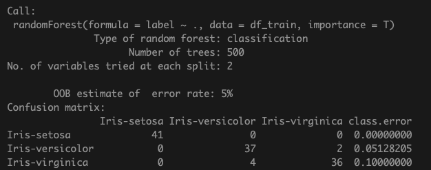
Confusion matrix shows a total of 6 mis-classifiations in the training data with out-of-bag error of 5%. The OOB error is estimated by calculating model accuracy using the data left out of the training set for a particular tree (since bootstrapping of samples is a characteristic of RF models).
df_e <- data.frame(err_rate = model$err.rate[,'OOB'],
                      n_trees=1:model$ntree)
ggplot(df_e, aes(x=n_trees, y=err_rate)) +
  geom_line() +
  labs(title='OOB error rate with respect to tree growth')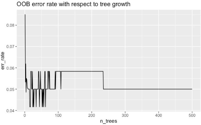
Next, fit the model to the validation set to see how the trained model generalize. Note that metrics such as confusion matrices can be made with the R package caret instead, which have dedicated functions.
df_pred_val <- predict(model, df_val, type='class')
table(df_pred_val, df_val$label)
Here, we achieve a classification accuracy of 93% on the validation data.
mean(df_pred_val == df_val$label)
The usefulness of the RF algorithm includes the ability to deduce which feature variables are important in predicting the target variable. There are two ways to assess variable importance:
Mean decrease in accuracy: the decrease in model accuracy if the variable values are randomly permuted.
Mean decrease in Gini impurity score: this measures how much including the given variable improves the purity of the nodes in the trees. Recall that in recursive partitioning, the split is chosen such that the impurity is minimized in the sub-partitions.
Since we set importance=TRUE in building the RF model, we can obtain the above measures easily.
importance(model)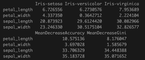
varImpPlot(model, type=1, main=NULL)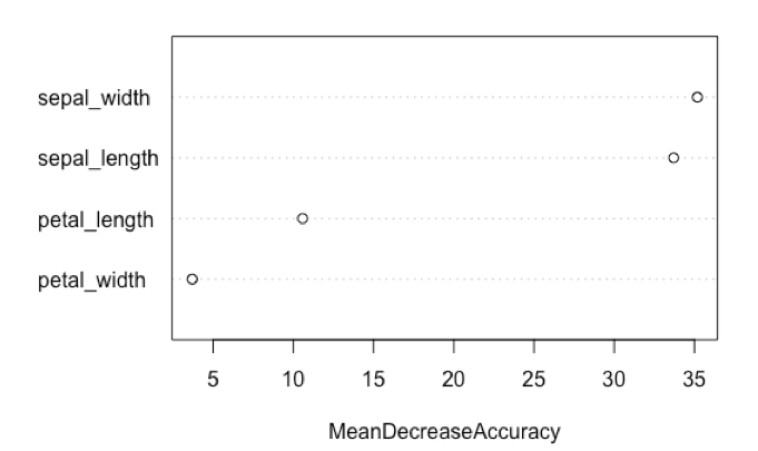
varImpPlot(model, type=2, main=NULL)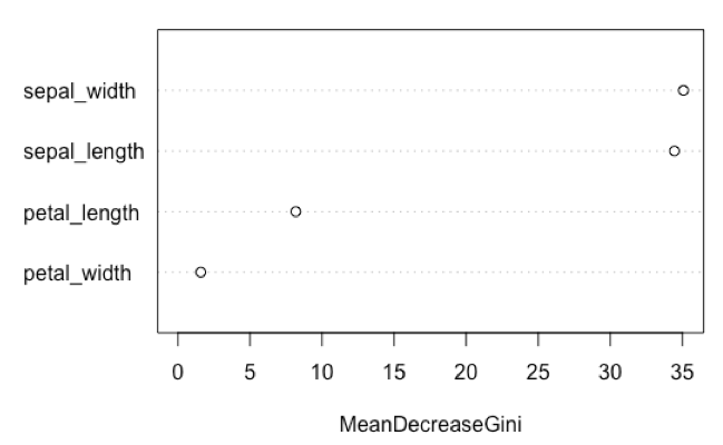
This result suggests that the characteristics of the iris sepal contribute more to the predictive ability of the model relative to the iris petals.
In summary:
RF models can be implemented in R using the randomForests package
Predictive models can be assessed using confusion matrices and validation set accuracy. Other measures such as ROC curves (sensitivity vs. specifcity curves) and their area-under-the-curve can also be used
OOB error indicates errors associated with bootstrapping of samples
Parameters of RF models include the growth of trees as well as number of aggregated variables during recursive partitioning
Variable importance can be assessed using mean decrease in accuracy per variable as well as decrease in Gini impurity scores