Natural Language Processing with Tensorflow, Keras
Jupyter notebook of following code and figures are available from my GitHub: https://github.com/snowoflondon.
Multi-layer neural networks such as MLPs typically involve data classification or regression problems. This could be useful when we are working with a dataset of typically numeric column values (i.e., called features or predictor variables) with a corresponding vector of target labels (i.e., called the target or response variables). A typical example of MLPs in say, regression, is prediction of housing prices using data such as location, number of bedrooms, etc.
However, a stacked network of 'dense layers', as shown in the previous post, may not be suitable for higher-order data. This is typically the case when the data we are working with are encoded in high-dimensional NumPy arrays (or 'tensors') as in the case of video data, image data, and sequence data. In 2D image processing, users typically use the concept of convolutional networks (convnets) to 'scan' a (n x n) window of pixels and identify patterns.
Natural language processing (NLP) handles sequence data - or more specifically, a sequence of words. This type of data is unique in a sense that the order of individual word (or character) is of importance - hence introducing a temporal aspect of our data dimension. How do we handle this?
Here, we will use a data set of Yelp reviews in order to build a predictive model wherein our target labels will reflect customer sentiment (i.e., positive or negative). This data set is publicly available here: https://www.kaggle.com/marklvl/sentiment-labelled-sentences-data-set. The goal will be to train a model using a small set of Yelp reviews and predict whether a new review is positive or negative.
First, load primary packages and the downloaded data set for preprocessing.
import pandas as pd
import tensorflow as tf
from tensorflow.keras import preprocessing
from tensorflow.keras.models import Sequential
from tensorflow.keras.layers import Flatten, Dense, Embedding
df = pd.read_csv('yelp_labelled.txt', names=['review', 'sentiment'], sep='\t')
df.head()Data looks like this:
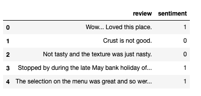
Before vectorizing the 'review' column (i.e., turning it into NumPy array so Keras can understand the data), it's a good idea to remove punctuations from the text.
import string
trans = str.maketrans('', '', string.punctuation)
processed = [a.translate(trans) for a in df['review']]
df2 = pd.concat([df, pd.Series(processed, name='review_processed')],axis=1)
df2 = df2.drop('review',axis=1)
df2.head()
New data looks like this:
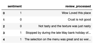
Separate the reviews from the labels:
y = df2['sentiment'].values
X = df2['review_processed'].values
X[1]
An example excerpt review will look like this:

As usual, we split the predictor variables into training and testing sets.
from sklearn.model_selection import train_test_split
X_train, X_test, y_train, y_test = train_test_split(X, y, test_size=0.20, random_state=42)
Now we need to do two things with the text data: first we must 'tokenize' it, then we need to pad them appropriately. A 'token' is essentially a unit in which text is broken down into (i.e, words or characters in most cases). In order to vectorize text data, we must first apply some sort of a tokenizer to break down our text data - likely in sentence or paragraph form - and then assign numeric vectors to the generated tokens.
from tensorflow.keras.preprocessing.text import Tokenizer
from tensorflow.keras.preprocessing.sequence import pad_sequences

max_words = 2000
max_len = 100

tokenizer = Tokenizer(num_words=max_words)
tokenizer.fit_on_texts(X_train)

X_train = tokenizer.texts_to_sequences(X_train)
X_test = tokenizer.texts_to_sequences(X_test)

X_train = pad_sequences(X_train, padding='post', maxlen=max_len)
X_test = pad_sequences(X_test, padding='post', maxlen=max_len)
The fit_on_texts method creates a vocabulary index based on the word frequency of input data. The text_to_sequences then transforms each text in texts to a sequence of integers. Padding sequences is necessary to make all sequences in a batch a standard length.
Another concept to introduce here, unique to NLPs, is the idea of embedding layers. Word embeddings are essentially low-dimensional, floating-point vectors that is learned from input text data. Word embeddings attempt to learn semantic relationships between words and essentially map the language input into a geometric space.
Embedding layers precede dense layers in a typical set-up, and can either be computed with the data at hand, or we can use a pre-computed embedding layer built from text databases. These pre-trained embedding layers are meant to capture the generic aspects of the language structure, which makes them applicable to more specific problems.
Here, we will use embedding data from GloVe (https://nlp.stanford.edu/projects/glove/). The pre-trained data we will use is based on data from Wikipedia.
For the sake of completion, we will first build an embedding layer from our data and use that for our model.
model = Sequential()
model.add(Embedding(10000, 8, input_length=max_len))
model.add(Flatten())
model.add(Dense(1, activation='sigmoid'))

model.compile(optimizer='rmsprop', loss='binary_crossentropy', metrics=['accuracy'])

model.summary()

hist = model.fit(X_train, y_train, epochs=10, batch_size=32, validation_split=0.2)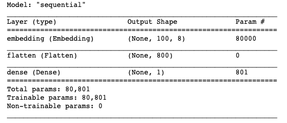
Making a quick function to plot our validation loss and accuracy across epochs:
import matplotlib.pyplot as plt
plt.style.use('fivethirtyeight')

def plot_measures(hist):

    plt.plot(hist.history['loss'])
    plt.plot(hist.history['val_loss'])
    plt.title('Model loss')
    plt.xlabel('Epoch')
    plt.ylabel('Loss')
    plt.legend(['Train', 'Val'], loc='upper right')
    plt.show()
    plt.clf()

    plt.plot(hist.history['accuracy'])
    plt.plot(hist.history['val_accuracy'])
    plt.title('Model accuracy')
    plt.xlabel('Epoch')
    plt.ylabel('Accuracy')
    plt.legend(['Train', 'Val'], loc='upper right')
    plt.show()
    plt.clf()
plot_measures(hist=hist)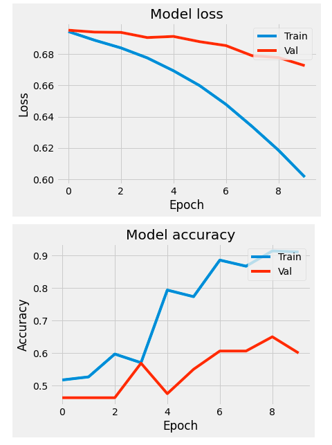
Validation acuracy is at around 60% after 10 iterations. Now we can use the downloaded GloVe embedding and see if performance improves:
import os
import numpy as np

gdir = '/Users/brianjmpark/Desktop/workspace/nlp/glove.6B/'

embeddings_index = {}
file = open(os.path.join(gdir, 'glove.6B.100d.txt'))

for line in file:
    values = line.split()
    word = values[0]
    coefs = np.asarray(values[1:], dtype='float32')
    embeddings_index[word] = coefs

file.close()

embedding_dim = 100
word_index = tokenizer.word_index

embedding_matrix = np.zeros((max_words, embedding_dim))
for word, i in word_index.items():
    if i < max_words:
        embedding_vector = embeddings_index.get(word)
        if embedding_vector is not None:
            embedding_matrix[i] = embedding_vector

model = Sequential()
embedding_layer = Embedding(max_words, embedding_dim, weights=[embedding_matrix], input_length=max_len , trainable=False)
model.add(embedding_layer)
model.add(Flatten())
model.add(Dense(32, activation='relu'))
model.add(Dense(1, activation='sigmoid'))

model.compile(optimizer='rmsprop', loss='binary_crossentropy', metrics=['accuracy'])

model.summary()

hist = model.fit(X_train, y_train, epochs=10, batch_size=32, validation_split=0.2)

plot_measures(hist=hist)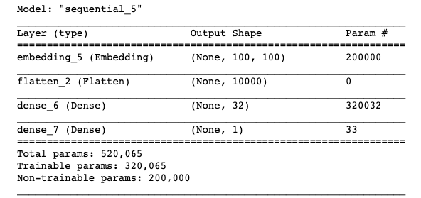
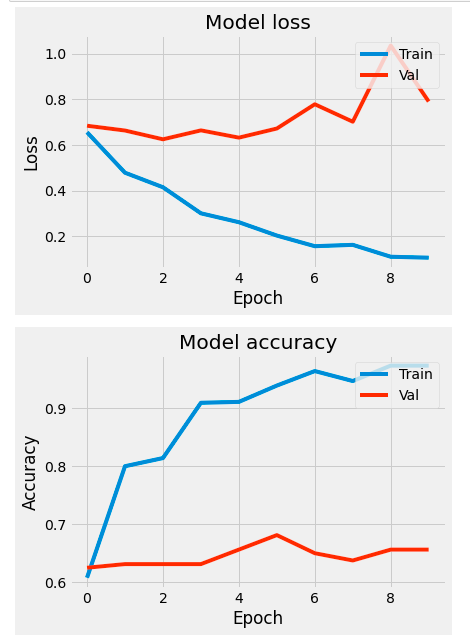
We seem to do a bit better in terms of our validation accuracy.
Instead of using a simple network as above, we can instead use a recurrent neural network (RNN). The central idea of RNN is the concept of memory. RNNs are built from past information and constantly updated as new information comes on. This is because RNNs essentially have an internal loop. It iterates through the data and maintains a state containing information relative to the past information. As you can image, this must be useful for sequential data where order matters - such as in the human language.
RNN algorithms such as LSTM (long short-termmemory) allows a way to carry information across many time-steps. It essentially saves information for later, while keeping state memory. We can implement a bi-directionality to LSTM, which allows us to essentially use two LSTM layers, which process sequence both chronologically and anti-chronologically. This is useful in NLP, as the importance of a word in a sentence isn't usually dependent on its relative position.
from tensorflow.keras.layers import LSTM, Bidirectional

model = Sequential()
embedding_layer = Embedding(max_words, embedding_dim, weights=[embedding_matrix], input_length=max_len , trainable=False)
model.add(embedding_layer)
model.add(Bidirectional(LSTM(64)))
model.add(Dense(1, activation='sigmoid'))

model.compile(optimizer='rmsprop', loss='binary_crossentropy', metrics=['accuracy'])

model.summary()

hist = model.fit(X_train, y_train, epochs=20, batch_size=32, validation_split=0.2)

plot_measures(hist=hist)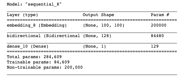
We've doubled the number of epochs to account for the bi-directionality of LSTM layer.
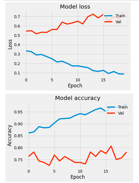
We can also add dropout layers and tune other hyper-parameters of the model in order to combat over-fitting. Here, we'll add dropout and lower the learning rate of our optimizer.
from tensorflow.keras.optimizers import RMSprop

model = Sequential()
embedding_layer = Embedding(max_words, embedding_dim, weights=[embedding_matrix], input_length=max_len , trainable=False)
model.add(embedding_layer)
model.add(Bidirectional(LSTM(64, dropout=0.2, recurrent_dropout=0.2)))
model.add(Dense(1, activation='sigmoid'))

model.compile(optimizer=RMSprop(learning_rate=0.0005), loss='binary_crossentropy', metrics=['accuracy'])

hist = model.fit(X_train, y_train, epochs=20, batch_size=64, validation_split=0.2)

plot_measures(hist=hist)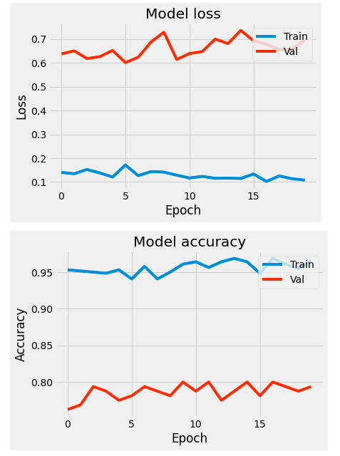
Don't forget to evaluate the model using testing data set to avoid validation data leak.
model.evaluate(X_test, y_test)[1]
We've achieved 79% accuracy despite using a relatively small training data set and just one layer of recurrent layer. Adding the number of neurons or stacking more layers may improve performance, but at the cost of computational load.
Here's how to feed new data into the predictive model, using a real review pulled from a local Olive Garden's yelp page.
example = "I got the chef's special and it got to my table cold. The soup was bland, meat was tough, and the waiter took half an hour to get our bill. I would not come here again."

example = [example.translate(trans)]

tokenizer.fit_on_texts(example)
example = tokenizer.texts_to_sequences(example)
example = pad_sequences(example, padding='post', maxlen=max_len)
model.predict(example)
Recall our activation function in the final layer is a sigmoid function, which outputs a probability value between 0 and 1. Our value is less than 0.5, hence we assign it the '0' label from our original label data - which corresponds to a negative review.
Finally, similar to how image data can harness 2D convnets to build a model, sequence data such as text can use convnets as well. In this case, time can be treated as a spatial dimension, similar to height and width of an image.
1D convnets can offer similar performance to RNNs, but at a smaller computational load. Similar to image processing in computer vision, convnets typically involve downsampling of data using a pooling layer.
from tensorflow.keras.layers import Conv1D, MaxPooling1D, GlobalMaxPooling1D

model = Sequential()
embedding_layer = Embedding(max_words, embedding_dim, weights=[embedding_matrix], input_length=max_len , trainable=False)
model.add(embedding_layer)
model.add(Conv1D(64, 7, activation='relu'))
model.add(MaxPooling1D(5))
model.add(Conv1D(64, 7, activation='relu'))
model.add(GlobalMaxPooling1D())
model.add(Dense(1, activation='sigmoid'))

model.summary()

model.compile(optimizer='rmsprop', loss='binary_crossentropy', metrics=['accuracy'])

hist = model.fit(X_train, y_train, epochs=10, batch_size=64, validation_split=0.2)

plot_measures(hist=hist)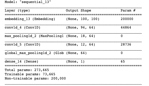
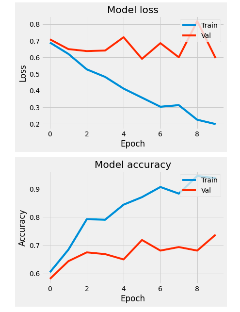
Here, our testing accuracy isn't as great as the one from RNN
model.evaluate(X_test, y_test)[1]
In summary:
Text data must undergo preprocessing prior to use in a neural network: this includes removing any HTML tags or punctuations, as well as tokenization and vectorization
Embedding layers give geometric representation in text data to give semantic meaning
RNNs use internal loops to maintain state representations of seen data
1D convnets are a cheaper alternative to RNNs, but performance may vary