Building a neural network with TensorFlow and Keras

Dec 27, 2020 · 6 min read

A neural network in a classification problem aims to learn underlying patterns in a feature-set to make predictions based on provided training data. A classic example of an ANN (artificial neural network) problem is image recognition, as in the case of the MNIST database of handwritten digits (http://yann.lecun.com/exdb/mnist/).

As with the case of other supervised ML algorithms in classification (e.g., support vector machines, k-nearest neighbors), the program is 'trained' using a set of data (called 'features', usually columns in a dataframe) with labeled targets (called the 'ground truth.') What a neural network does, is that it makes predictions based on provided features by assigning 'weights' and calculates the amount of deviation from the ground truth. This deviation can often be measured as the accuracy of the model, sometimes calculated as the mean standard error. The model then 'backpropagates' to minimize the loss and assign adjusted weights to make the next subsequent predictions.

The notion of the feed-forward mechanism (i.e., assignment of weights to features in order to make predictions) and backpropagation (i.e., minimization of the loss function) is at the core of training neural networks.

The assignment of weights to each feature can be thought of as vector arithmetic. More specifically, our 'input' - an array of vectors from a dataframe - and our weight come together in a vector dot product. This is a 'tensor' operation, where a tensor is loosely defined as a container of data.

In the most common examples, we work with 2-dimensional (2D) tensors, which can be expressed as an Numpy array in Python with attribute ndim = 2. These are essentially an array of vectors, where its axes are: the samples axis (i.e., rows from a dataframe) and the feature axis (i.e., columns from a dataframe). A scalar value is said to be a 0D tensor, whereas image data are stored in 4D tensors (samples, height, width, and channels).

Neural networks have 'layers' where these tensor operations take place. Each layer is associated with:

an activation function, which transforms the output of each layer so that it's easier for the model to learn complex patterns in our data
'neurons' or nodes, where tensor operations take place
optionally, some kind of a measure against overfitting to the training data, such as a regularization factor

In the simplest example, an ANN can have an input layer, a middle hidden layer, and an output layer. The input layer must accept a tensor of shape equal to the input data, and the output layer must produce a tensor of shape representative of the target labels.

TensorFlow, using Keras API, can handle building such a network.

Here, a multi-label classification problem is shown, with the dataset provided by the UCI machine learning repository. This dataset in particular assigns an integer value indicating the quality of red wine, with each column as dependent variables (e.g., acidity, pH, etc.).

Step by step:

First we load the appropriate modules.

import pandas as pd
import numpy as np
import tensorflow as tf
from tensorflow.keras.models import Sequential
from tensorflow.keras.layers import Dense
from sklearn.model_selection import train_test_split
from sklearn import preprocessing
from sklearn.metrics import accuracy_score
import matplotlib.pyplot as plt

We load our red wine dataset and split the dataframe into its feature-set (i.e., the dependent variables) and our target labels.

df = pd.read_csv('winequality-red.csv', sep=';')
y = df.select_dtypes('int').values
X = df.select_dtypes(exclude='int').values

It is important to preprocess our features. This is especially important in cases where the values across different columns are hetereogenous in their value ranges (e.g., one feature ranges from 0-1 whereas another ranges from 300-500). It's also recommended not to feed into a neural network data that can take large values. The min-max scaler from sklearn normalizes the data such that every value is between 0 and 1.

min_max_scaler = preprocessing.MinMaxScaler()
X_scale = min_max_scaler.fit_transform(X)

We now split our data into training and testing data. The testing data will not be seen by our model during the training phase and will only be used to evaluate our model accuracy after the training phase. It is vital that the model is tested using never-before-seen data.

X_train, X_test, y_train, y_test = train_test_split(X_scale, y, test_size = 0.2, random_state = 4)

The target labels are encoded. Usually, one-hot encoding is done on labels that are non-numeric values (e.g., strings) in order to associate a unique integer index with each unique label. This will return a vector whose size equals to the size of the number of unique labels.

y_train_sequential = tf.keras.utils.to_categorical(y_train)

We now build the network of three layers. The input and the middle layer will have 64 neurons with the rectified linear unit activation function. The first layer takes the input of shape (11,) since the feature axis in our input tensor (i.e., number of features) equals to 11. The output layer will use the softmax activation function to produce a probability distribution over the number of different output labels, where output[n] equals to the probability that the sample belongs to class n.

model = Sequential([
  Dense(64, activation='relu', input_shape(11,)),
  Dense(64, activation='relu'),
  Dense(y_train_categorical.shape[1], activation='softmax')
])

The model is now compiled using the parameters we've mentioned earlier - a measurement of how well our model is doing (i.e., accuracy), a function the model will use to measure its performance on training data (i.e., loss), and an optimizer used for backpropagation.

model.compile(optimizer='rmsprop', loss='categorical_crossentropy', metrics=['accuracy'])

We now train our model and store the results. Each iteration over the entire training data is called an epoch. This process will therefore iterate a thousand times.

history = model.fit(X_train, y_train_categorical, batch_size=512, epochs=1000, validation_split=0.2)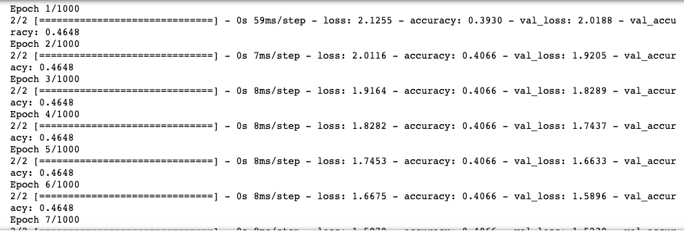

We plot the model loss and accuracy on the training and validation data with respect to the iterations.

plt.style.use('fivethirtyeight)
plt.plot(history.history['loss'])
plt.plot(history.history['val_loss'])
plt.title('Model loss')
plt.xlabel('Epoch')
plt.ylabel('Loss')
plt.legend(['Train', 'Val'], loc='upper right')
plt.show()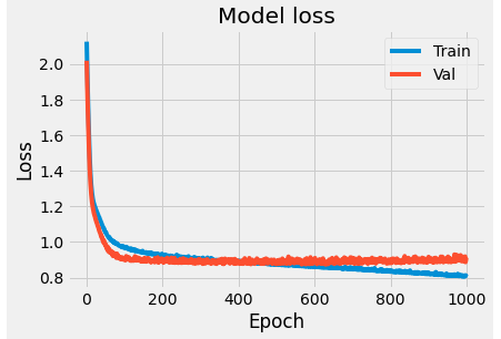

plt.plot(history.history['accuracy'])
plt.plot(history.history['val_accuracy'])
plt.title('Model accuracy')
plt.xlabel('Epoch')
plt.ylabel('Accuracy')
plt.legend(['Train', 'Val'], loc='upper right')
plt.show()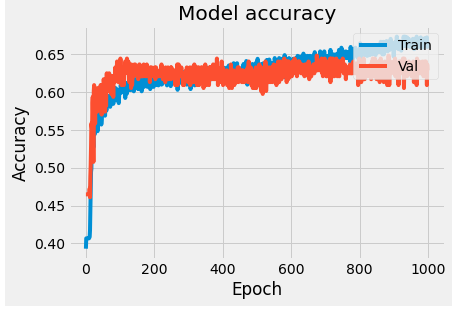

As you can see, the accuracy on validation data plateaus after a couple hundred epochs and lags behind the accuracy on the training data. This behaviour is as known as overfitting, where the model is unable to generalize to unknown data. In order to mitigate this behaviour, we can add dropout layers (where we essentially 'turn off' a select percentage of neurons in a layer) or add regularization factors (essentially penalties to overcome overfitting).

Adding regularization factors:

from tensorflow.keras import regularizers



model = Sequential([
  Dense(64, activation='relu', input_shape(11,), kernel_regularizer=regularizers.l2(0.001)),
  Dense(64, activation='relu', kernel_regularizer=regularizers.l2(0.001)),
  Dense(y_train_categorical.shape[1], activation='softmax')
])

model.compile(optimizer='rmsprop', loss='categorical_crossentropy', metrics=['accuracy'])

history = model.fit(X_train, y_train_categorical, batch_size=512, epochs=1000, validation_split=0.2)



plt.style.use('fivethirtyeight)
plt.plot(history.history['loss'])
plt.plot(history.history['val_loss'])
plt.title('Model loss')
plt.xlabel('Epoch')
plt.ylabel('Loss')
plt.legend(['Train', 'Val'], loc='upper right')
plt.show()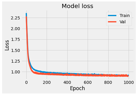

plt.plot(history.history['accuracy'])
plt.plot(history.history['val_accuracy'])
plt.title('Model accuracy')
plt.xlabel('Epoch')
plt.ylabel('Accuracy')
plt.legend(['Train', 'Val'], loc='upper right')
plt.show()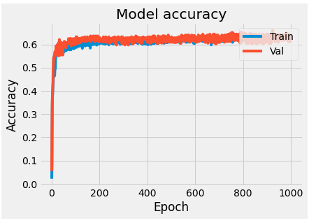

Adding dropout:

from tensorflow.keras.layers import Dropout

model = Sequential([
  Dense(64, activation='relu', input_shape(11,)),
  Dropout(0.5),
  Dense(64, activation='relu'),
  Dropout(0.5),
  Dense(y_train_categorical.shape[1], activation='softmax')
])

model.compile(optimizer='rmsprop', loss='categorical_crossentropy', metrics=['accuracy'])

history = model.fit(X_train, y_train_categorical, batch_size=512, epochs=1000, validation_split=0.2)



plt.style.use('fivethirtyeight)
plt.plot(history.history['loss'])
plt.plot(history.history['val_loss'])
plt.title('Model loss')
plt.xlabel('Epoch')
plt.ylabel('Loss')
plt.legend(['Train', 'Val'], loc='upper right')
plt.show()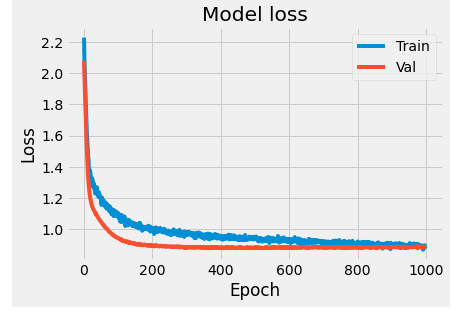

plt.plot(history.history['accuracy'])
plt.plot(history.history['val_accuracy'])
plt.title('Model accuracy')
plt.xlabel('Epoch')
plt.ylabel('Accuracy')
plt.legend(['Train', 'Val'], loc='upper right')
plt.show()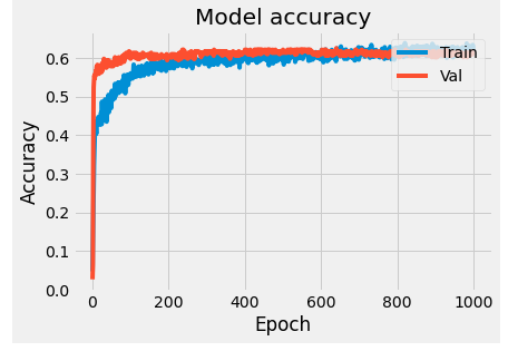

Finally, to evaluate the model accuracy on our testing data:

results = model.evaluate(X_test, y_test_categorical)

We have around 63% accuracy on classifying wine quality based on our dataset, with just using one hidden layer.